First Steps in Machine Learning with Microsoft Azure. Part 1

Machine learning is applied to a wide range of business tasks – from detecting frauds to selecting the target audience and product recommendations, as well as monitoring production in real time, analyzing the tonality of texts and medical diagnostics. It can take over the tasks that can not be performed manually due to the huge amount of data to be processed. In case of a large set of data, machine learning sometimes reveals non-obvious dependencies that cannot be detected by an arbitrary rigorous manual examination. In this case, the combination of the set of such “weak” relations gives perfectly functioning forecasting mechanisms.

The process of learning from the data and the subsequent application of the knowledge to justify future decisions is an extremely powerful tool. Machine learning quickly turns into the engine of a modern, data-driven economy.

In recent years, machine learning (‘ML’) has turned into a large business – companies use it to earn money. Applied research is rapidly developing both in industrial and academic environments, and curious developers everywhere are looking for an opportunity to raise their experience level in this field. Nevertheless, the emerging demand far exceeds the speed of the appearance of good techniques and tools.

In this post, we would like to describe how you can use Microsoft Azure Machine Learning Studio to build machine learning models, as well as what problems you might encounter while using Azure ML and how to get around them.

Tools and Basics

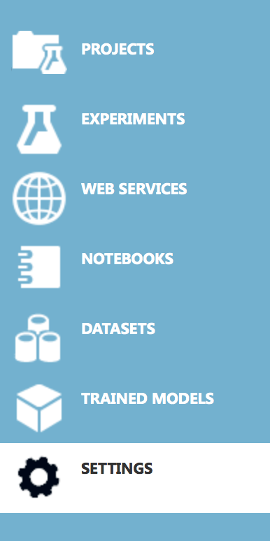
Here we have several tabs:

• Projects – represent groups of experiments
• Experiments – similar to the ipython notebooks
• Web services
• Notebooks – ipython notebooks
• Saved data
• Models
• Settings

Pay attention to the settings tab:

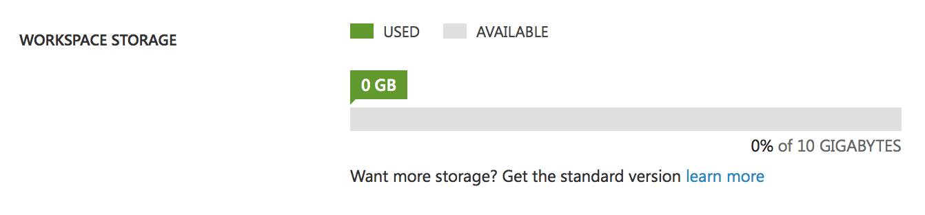
This is our spare space for data, models, and experiments. 10 GB storage is one of the limitations of the free account. It might seem that it is quite enough, but remember that Studio stores all the intermediate data of the experiments, that is, if you have an experiment with a 1Gb data volume, then after several changes or the launch of the experiment your disk will be full and you will have to clear the intermediate data. In a paid account this restriction does not exist, you will have an almost infinite disk. Also, there is one more difference between accounts: Free account can only run 1 experiment at a time, that is, you will have only one thread, whereas Premium account provides the opportunity to run many experiments simultaneously or to create parallel processes within one experiment.

Creating your first experiment

Let’s create an experiment and get acquainted with the process of building a model.

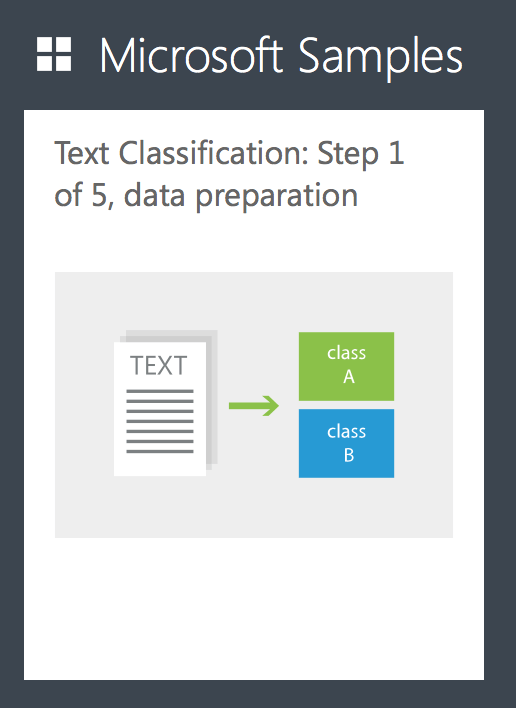
Select – add the experiment and find an example of Text Classification.

Studio will create an experiment and automatically download the data.

Here is our first experiment:

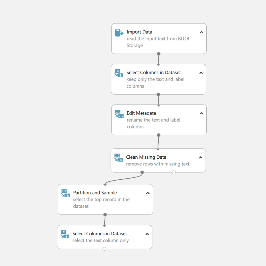
Let’s see what happens here. In fact, we see the first task that ML has to deal with, the processing and preparation of data.

1. Loading data (in our case they are stored in Azure Blob)
2. Selecting the required fields
3. Editing metadata
4. Deleting data with missing fields
5. Split of data

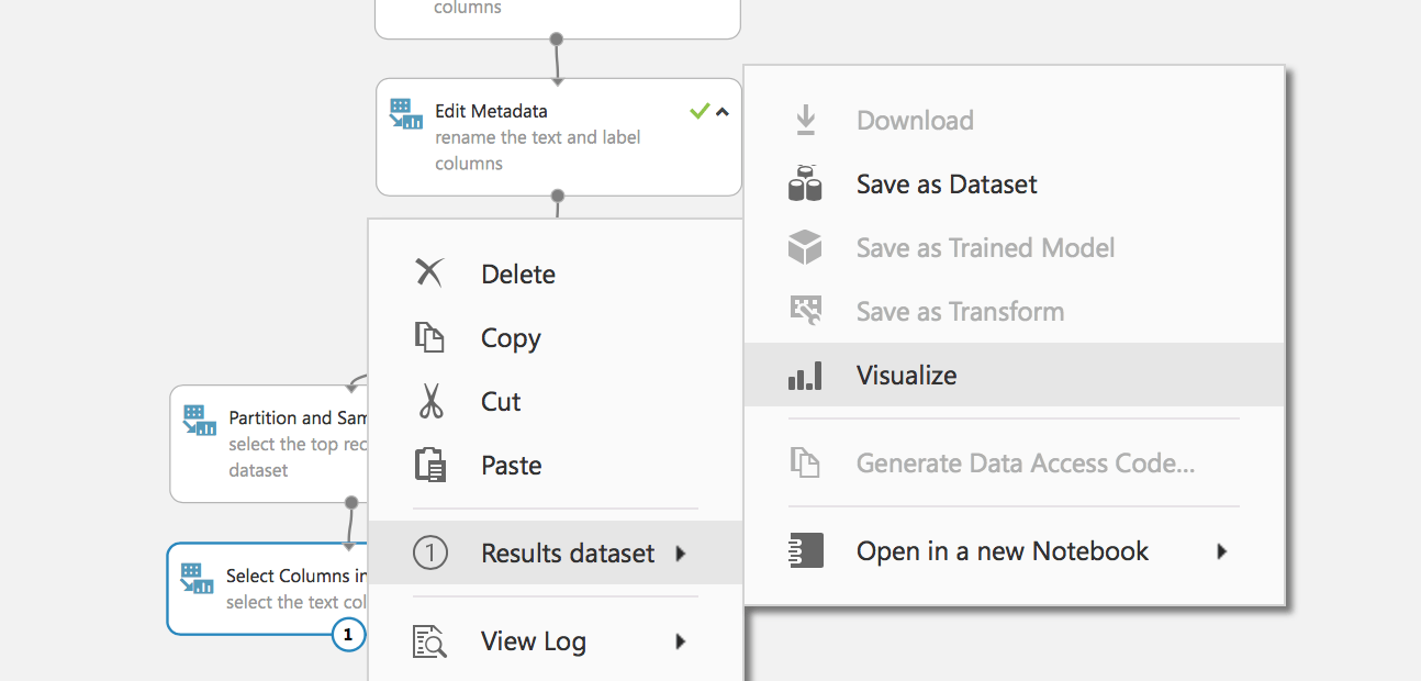
Run the experiment and examine the collected data:

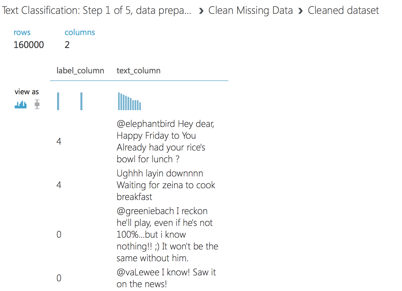
We have prepared the data and are ready to proceed to the next step. Load the following experiment – Text Classification: Step 2 of 5, text preprocessing

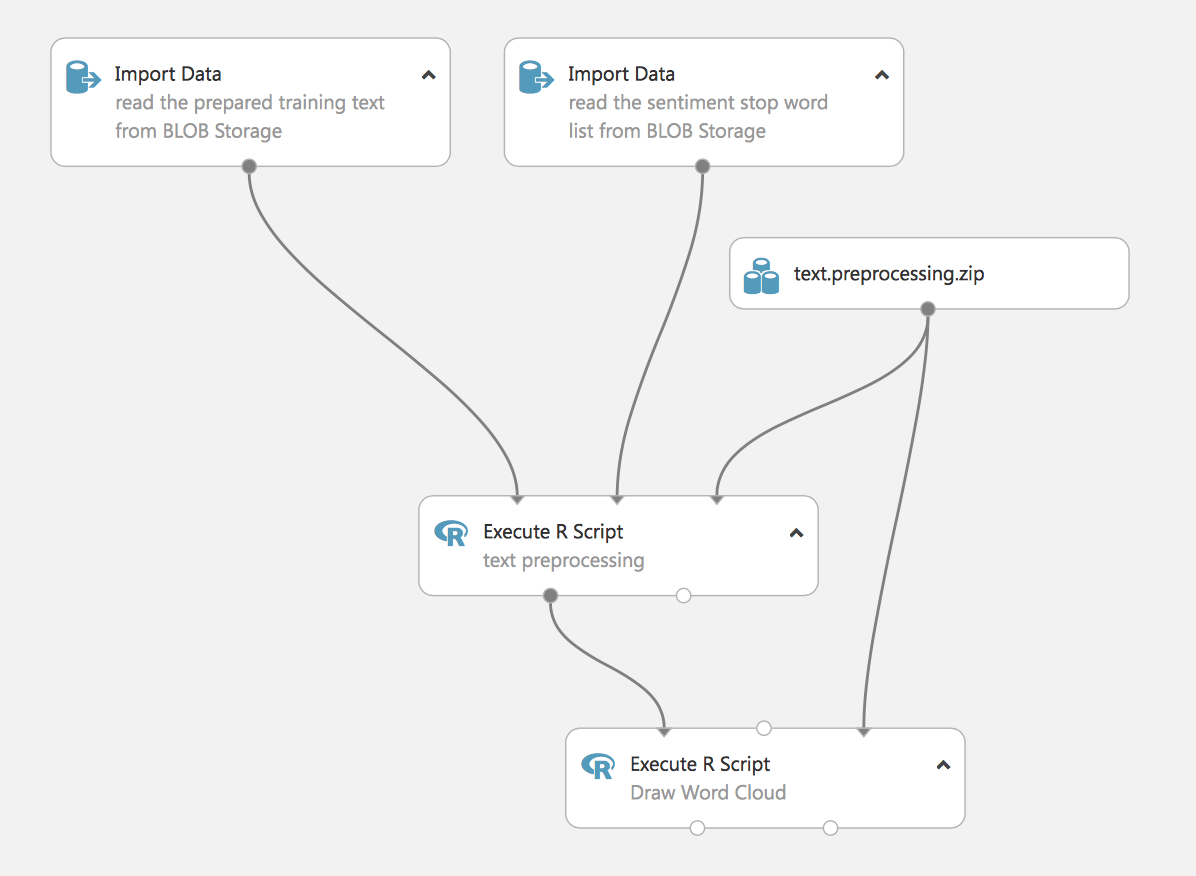
At this stage, we load the data and process it. This experiment uses scripts in R to remove stop words (we also load them from blob).

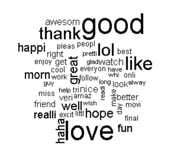
The final step is to visualize word cloud. This is an experiment with practical value, it demonstrates Studio’s ability to use R scripts for ML tasks, and we can also embed Python scripts into the process. Further, in the article, we’ll show an example of processing text using standard Studio methods.

Let’s run the experiment and study the results.

At the output of the first R script, we see the drafted text.

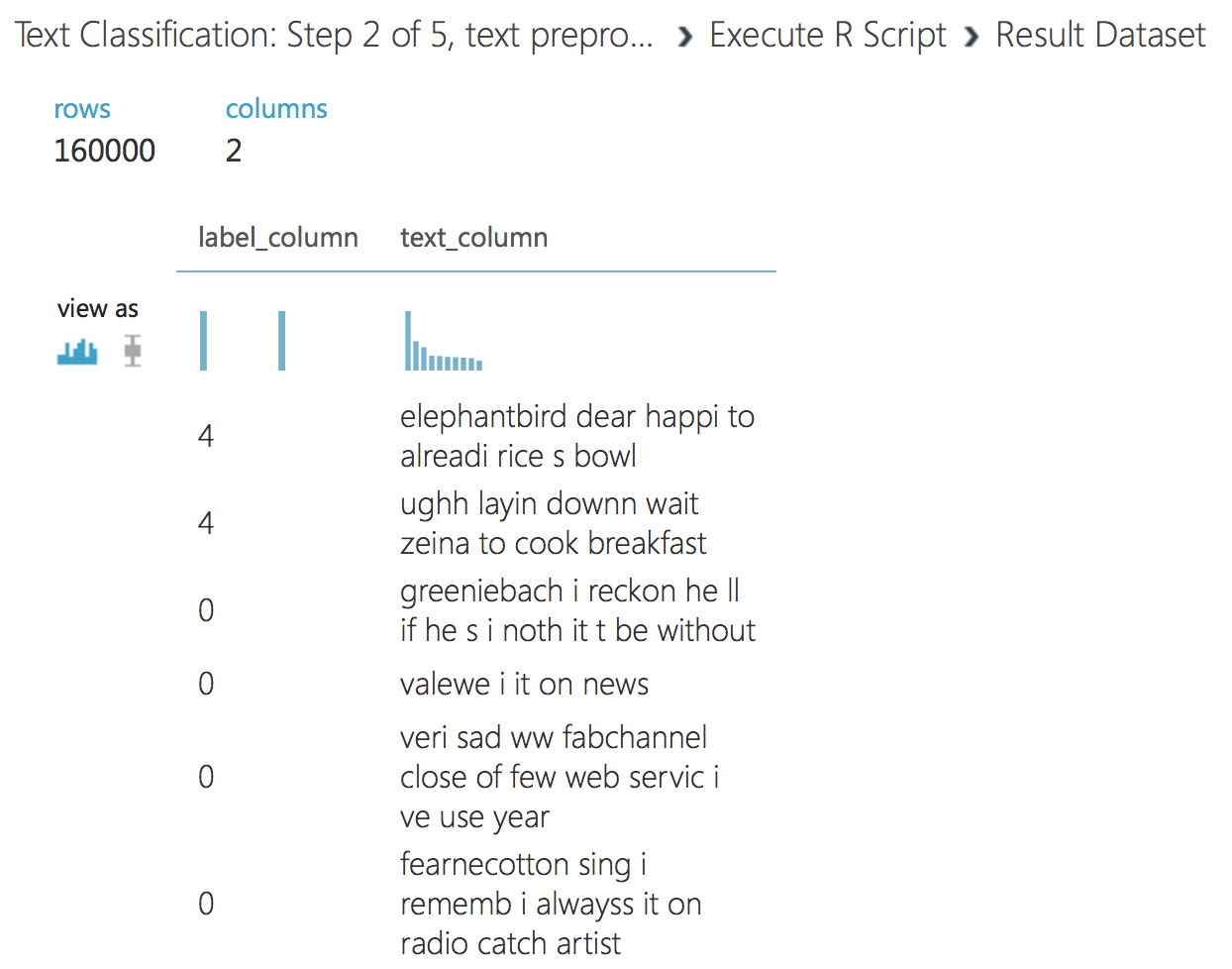
The second script generates a cloud of words. This is sometimes necessary for the visibility of data.

Let’s move on, create the next experiment, it uses data from the first script of the previous experiment.

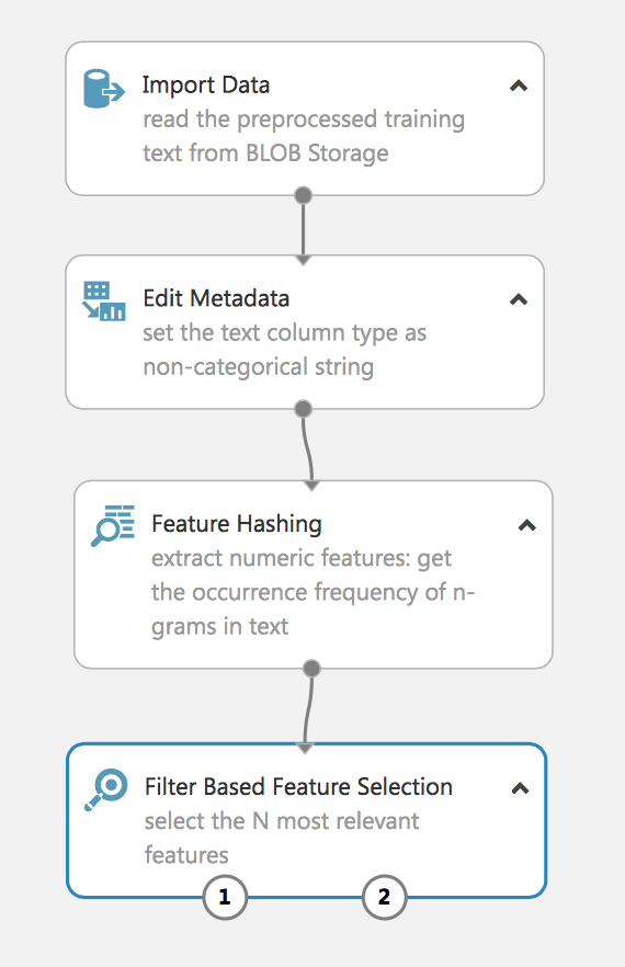
The experiment extracts the N-grams from the text data using the Term Frequency method and then selects the most relevant ones. A similar process is often used to process Natural Language.

Let’s check the received data:

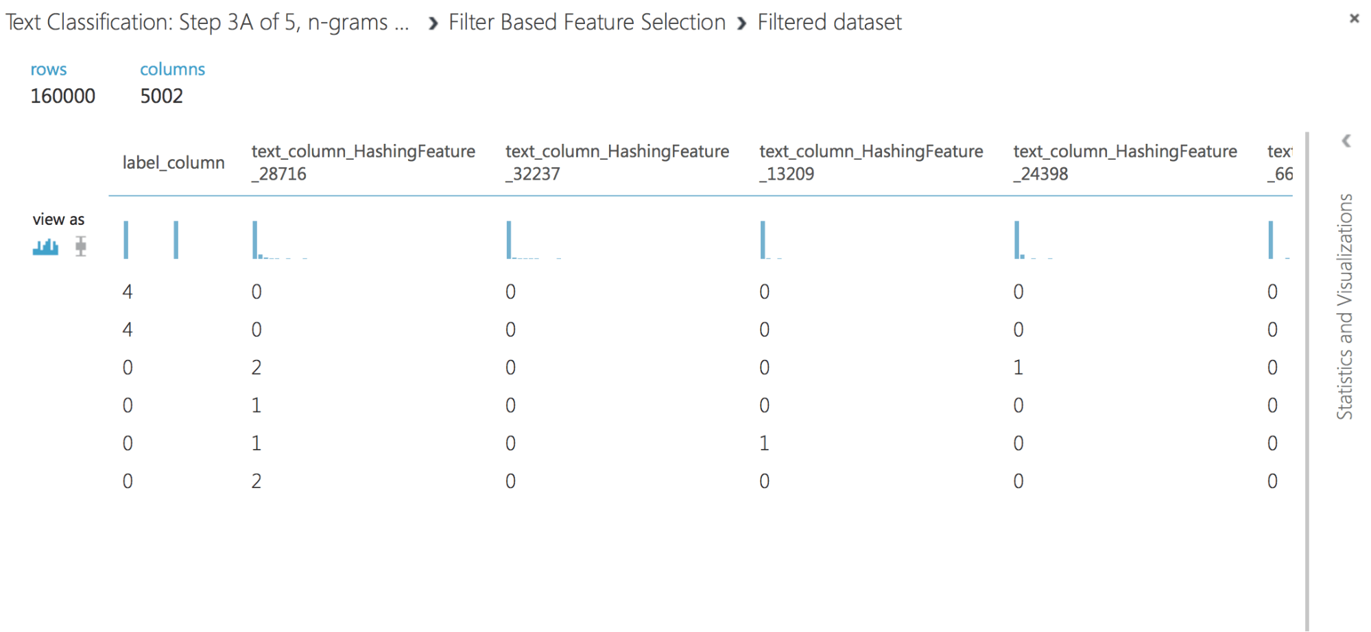
As you can see, we successfully extracted the hashing feature from the text data and filtered the most relevant one. If you do not use a filter, then on a sample of 160,000 we will get a vector in tens of thousands features, and this will complicate the task of learning the model and can lead to retraining.

The following experiment demonstrates another approach for processing NL-TF-IDF (Term Frequency Inverse Document Frequency).

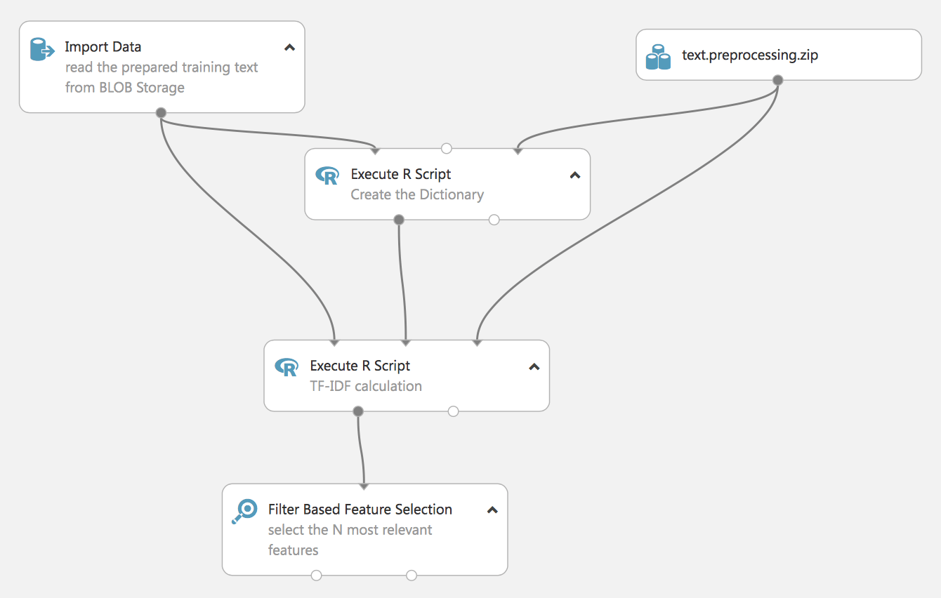
It is also built in R language, later we will show how it can be done with standard Studio tools.

The result of the experiment will also be the most relevant feature vector, but built on a previously created dictionary (that is also based on our data), it is not shown in the experiment – but do not forget to save the dictionary, as it will be needed to prepare real data afterward.

Let’s build a flow learning model.

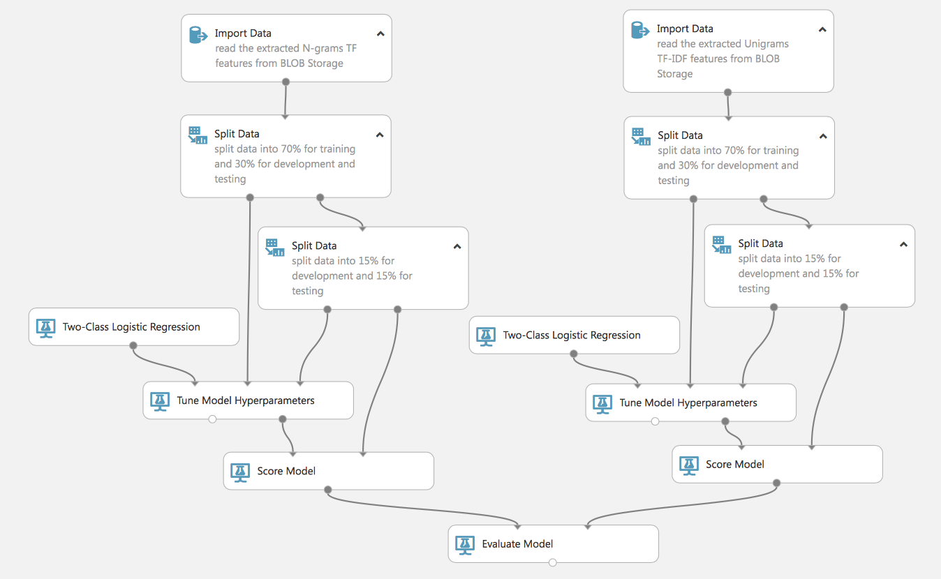
As you see, we can build complex and parallel processes (remember that on the free account this will all be done sequentially, on the paid account – simultaneously, this reduces the learning time of the models). Similarly, such a flow will allow us to train 2 models and compare their effectiveness, it is very convenient for choosing the most suitable models or methods of data preparation.

Let’s take a closer look at this process. At the start, it has 2 sets of prepared data using various methods of TF, TF-IDF. Both of these sets we divide into training and test data (that do not participate in the training of the model and will be used to assess its quality). Notice that we share the test dataset a second time, this is necessary for the next step.

We declare a model (in this example we will use Logistic Regression), but for greater efficiency, we will include the closest analog of GridSearchCV in the process of Tune Model Hyperparameters (for sklearn libraries familiar to python). That is, we do not rigidly set the parameters of the model, but set the range parameters and pass them to the Tune Model block, which will select the most effective ones during the training of the model. It is for this block that we need a second set of test data.

Let’s run this flow and examine the results.

Results of Tune Model:

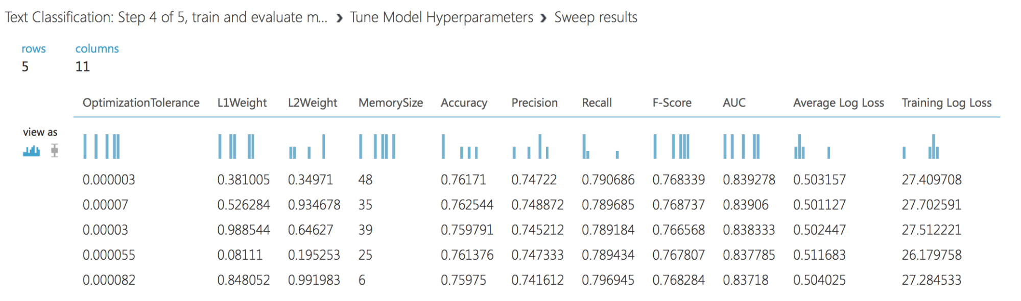
And the parameters of the best model (it goes further for evaluation):

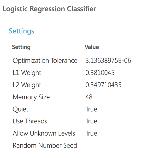
As we see the parameters of the models are identical. Let’s compare quality. This is the ROC chart for two models:

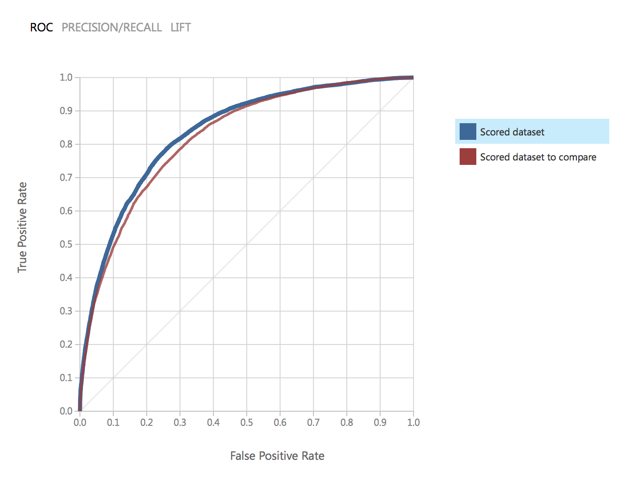
As can be noted, the results of both models are very close and satisfy our accuracy.

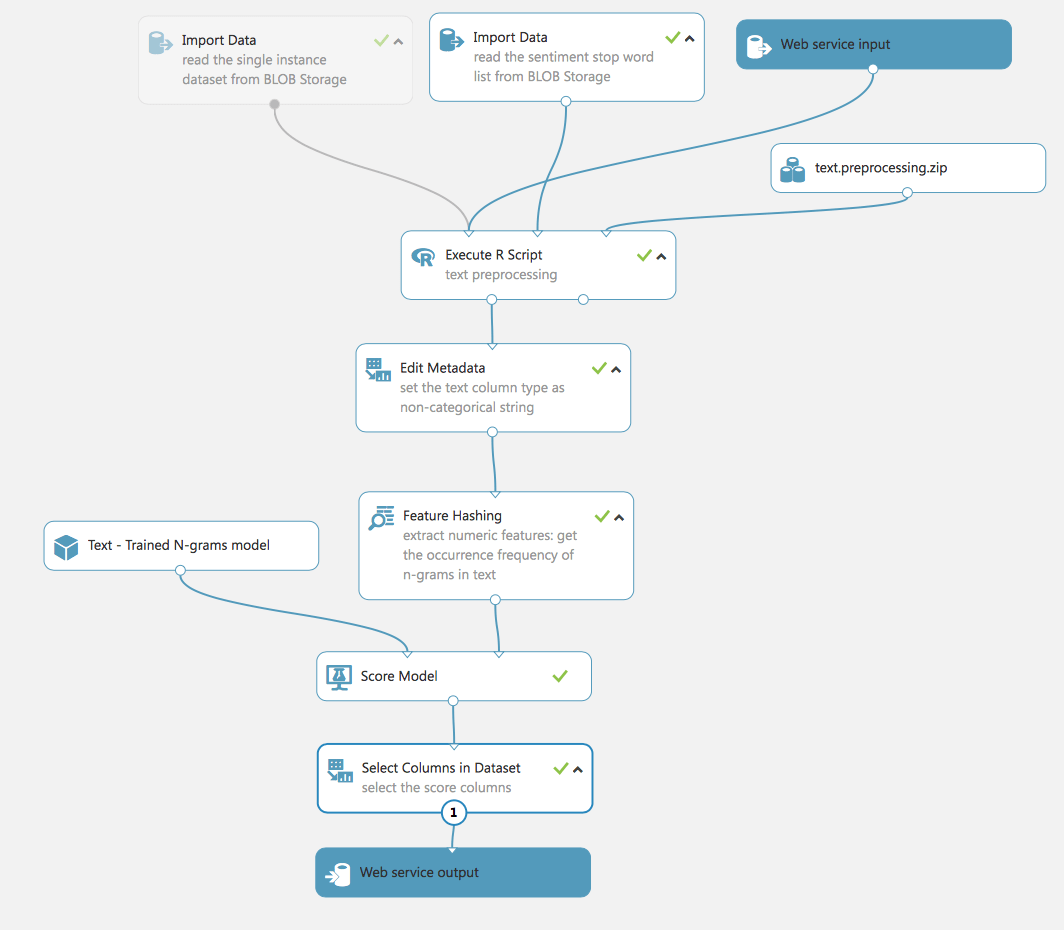
Let’s go ahead, and build an experiment that will allow using the model for real data (for example, coming through the Web Service).

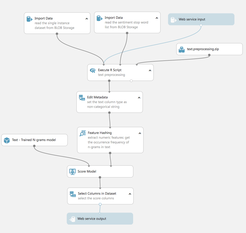
This experiment uses a model trained by the TF process. For real data, we repeat the same steps as for the process of preparing the training data: data cleaning, extraction features, filter.

Thus it should be emphasized, that the experiment has 3 inputs: data for testing (1 line from the original dataset), the dataset with stop words for preparing the text (we already used it in previous experiments) and Web Service input.

Web Service input and Web Service output is exactly what turns our experiment into a real project available for use. By switching the experiment to Web Service View, we can deploy the experiment and make it available from outside the Studio.

Going deeper

In this part of the article, we took a brief look at the example of creating a model and got acquainted with the most important steps in ML: data preparation, selection of trait, model training (selection of model parameters), and final evaluation of results (AUC, Precision, Recall, etc. )

In the next part, we will consider the process of creating a model for solving a real problem, on real data and to be applied in a real project.